6月13日
8.3 階層正規モデル
\[\begin{align*} \phi_j = \{\theta_j, \sigma^2\}, \quad p(y \mid \phi_j) = \mathrm{normal}(\theta_j, \sigma^2) \quad \text{(グループ内モデル)} \\ \psi = \{\mu, \tau^2\}, \quad p(\theta_j \mid \psi) = \mathrm{normal}(\mu, \tau^2) \quad \text{(グループ間モデル)} \end{align*}\] \[\begin{align*} \frac{1}{\sigma^2} &\sim \mathrm{gamma}(\frac{\nu_0}{2}, \frac{\nu_0 \sigma_0^2}{2}) \\ \frac{1}{\tau^2} &\sim \mathrm{gamma}(\frac{\eta_0}{2}, \frac{\eta_0 \tau_0^2}{2}) \\ \mu &\sim \mathrm{normal}(\mu_0, \gamma_0^2) \end{align*}\]事後推論
\[\begin{align*} p(\theta_1, \ldots , \theta_m, \mu,\tau^2,\sigma^2 \mid y_1,\ldots ,y_m ) &\propto p(\mu,\tau^2,\sigma^2)\times p(\theta_1, \ldots , \theta_m\mid\mu,\tau^2,\sigma^2)\times p(y_1,\ldots ,y_m\mid\theta_1, \ldots , \theta_m, \mu,\tau^2,\sigma^2) \\ &= p(\mu)p(\tau^2)p(\sigma^2)\left\{\prod_{j=1}^m p(\theta_j\mid\mu,\tau^2)\right\}\left\{\prod_{j=1}^m\prod_{i=1}^{n_j} p(y_{i,j}\mid\theta_j,\sigma^2)\right\} \end{align*}\]$\mu$と$\tau^2$の完全条件付き分布
\[\begin{align*} p(\mu\mid\theta_1,\ldots,\theta_m,\tau^2,\sigma^2,y_1,\ldots,y_m ) &\propto p(\mu)\prod p(\theta_j\mid\mu,\tau^2) \\ p(\tau^2\mid\theta_1,\ldots,\theta_m,\mu,\sigma^2,y_1,\ldots,y_m ) &\propto p(\tau^2)\prod p(\theta_j\mid\mu,\tau^2) \end{align*}\]一変量正規モデルにおける完全条件付き分布と同様に考えて
\[\begin{align*} \{\mu\mid\theta_1,\ldots,\theta_m,\tau^2\} &\sim \mathrm{normal}\left(\frac{\frac{m\bar{\theta}}{\tau^2}+\frac{\mu_0}{\gamma_0^2}}{\frac{m}{\tau^2}+\frac{1}{\gamma_0^2}}, \left(\frac{m}{\tau^2}+\frac{1}{\gamma_0^2}\right)^{-1}\right) \\ \{1/\tau^2\mid\theta_1,\ldots,\theta_m,\mu\} &\sim \mathrm{gamma}\left(\frac{\eta_0+m}{2}, \frac{\eta_0\tau_0^2+\sum(\theta_j-\mu)^2}{2}\right) \end{align*}\]$\theta_j$の完全条件付き分布
\[\begin{align*} p(\theta_j\mid\mu,\tau^2,\sigma^2,y_1,\ldots,y_m ) &\propto p(\theta_j\mid\mu,\tau^2)\prod_{i=1}^{n_j} p(y_{i,j}\mid\theta_j,\sigma^2) \end{align*}\]同様に
\[\begin{align*} \{\theta_j\mid y_{1,j},\ldots,y_{n_j,j},\mu,\tau^2,\sigma^2\} &\sim \mathrm{normal}\left(\frac{\frac{n_j\bar{y_j}}{\sigma^2}+\frac{\mu}{\tau^2}}{\frac{n_j}{\sigma^2}+\frac{1}{\tau^2}}, \left(\frac{n_j}{\sigma^2}+\frac{1}{\tau^2}\right)^{-1}\right) \end{align*}\]$\sigma^2$の完全条件付き分布
\[\begin{align*} p(\sigma^2\mid\theta_1,\ldots,\theta_m,y_1,\ldots,y_m ) &\propto p(\sigma^2)\prod_{j=1}^m\prod_{i=1}^{n_j} p(y_{i,j}\mid\theta_j,\sigma^2) \\ &\propto (\sigma^2)^{-\nu_0/2+1}e^{-\frac{\nu_0\sigma_0^2}{2\sigma^2}}(\sigma^2)^{-\sum n_j/2}e^{-\frac{\sum\sum(y_{i,j}-\theta_j)^2}{2\sigma^2}} \end{align*}\]m個のグループから$\sigma^2$の情報を得ていること以外は一変量正規モデルにおける完全条件付き分布と同様なので
\[\begin{align*} \{1/\sigma^2\mid\theta,y_1,\ldots,y_m\} &\sim \mathrm{gamma}\left(\frac{\nu_0+\sum_{j=1}^m n_j}{2}, \frac{\nu_0\sigma_0^2+\sum_{j=1}^m\sum_{i=1}^{n_j}(y_{i,j}-\theta_j)^2}{2}\right) \end{align*}\]8.4 例:米国公立学校における数学試験
すべての$\theta_j$がある共通の値$\theta_0$と等しい場合、各標本平均の期待値は$E[\bar{Y_j}\mid\theta_j,\sigma^2]=\theta_j=\theta_0$となるが、分散は$Var[\bar{Y_j}\mid\sigma^2]=\sigma^2/n_j$のようにサンプルサイズに依存する形になるため、サンプルサイズが大きいグループの標本平均値は$\theta_0$に非常に近くなり、サンプルサイズが小さいグループの平均値は$\theta_0$から極端に大きい値も小さい値も取りうる
Y <- dget("Y.school.mathscore.txt")
## weakly informative priors
nu0<-1 ; s20<-100
eta0<-1 ; t20<-100
mu0<-50 ; g20<-25
## starting values
m<-length(unique(Y[,1]))
n<-sv<-ybar<-rep(NA,m)
for(j in 1:m)
{
ybar[j]<-mean(Y[Y[,1]==j,2])
sv[j]<-var(Y[Y[,1]==j,2])
n[j]<-sum(Y[,1]==j)
}
theta<-ybar
sigma2<-mean(sv)
mu<-mean(theta)
tau2<-var(theta)
## setup MCMC
set.seed(1)
S<-5000
THETA<-matrix( nrow=S,ncol=m)
MST<-matrix( nrow=S,ncol=3)
## MCMC algorithm
for(s in 1:S)
{
# sample new values of the thetas
for(j in 1:m)
{
vtheta<-1/(n[j]/sigma2+1/tau2)
etheta<-vtheta*(ybar[j]*n[j]/sigma2+mu/tau2)
theta[j]<-rnorm(1,etheta,sqrt(vtheta))
}
#sample new value of sigma2
nun<-nu0+sum(n)
ss<-nu0*s20;for(j in 1:m){ss<-ss+sum((Y[Y[,1]==j,2]-theta[j])^2)}
sigma2<-1/rgamma(1,nun/2,ss/2)
#sample a new value of mu
vmu<- 1/(m/tau2+1/g20)
emu<- vmu*(m*mean(theta)/tau2 + mu0/g20)
mu<-rnorm(1,emu,sqrt(vmu))
# sample a new value of tau2
etam<-eta0+m
ss<- eta0*t20 + sum( (theta-mu)^2 )
tau2<-1/rgamma(1,etam/2,ss/2)
#store results
THETA[s,]<-theta
MST[s,]<-c(mu,sigma2,tau2)
}
mcmc1<-list(THETA=THETA,MST=MST)
library(ggplot2)
library(dplyr)
library(tidyr)
MST <- as.data.frame(mcmc1$MST)
colnames(MST) <- c("mu", "sigma2", "tau2")
S <- nrow(MST)
MST$chunk <- cut(1:S, breaks=10, labels=FALSE)
MST$iteration <- 1:S
chunk_labels <- MST %>%
group_by(chunk) %>%
summarise(mid_iter = median(iteration))
MST_long <- MST %>%
pivot_longer(cols = c(mu, sigma2, tau2), names_to = "parameter", values_to = "value") %>%
left_join(chunk_labels, by = "chunk")
# プロット
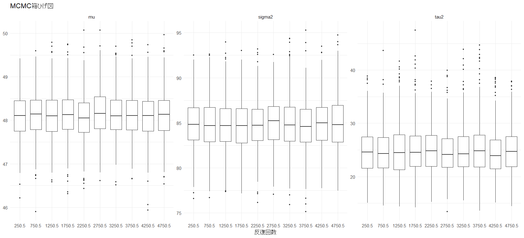
print(ggplot(MST_long, aes(x = factor(mid_iter), y = value)) +
geom_boxplot(outlier.size = 1, width = 0.7) +
facet_wrap(~ parameter, scales = "free_y", nrow = 1,
labeller = labeller(parameter = c(mu = expression(mu),
sigma2 = expression(sigma^2),
tau2 = expression(tau^2)))) +
labs(x = "反復回数", y = NULL,
title = expression("MCMC箱ひげ図")) +
theme_minimal(base_size = 14))
library(coda)
mcmc_MST <- as.mcmc(MST[, c("mu", "sigma2", "tau2")])
# 有効サンプルサイズの計算
ess <- effectiveSize(mcmc_MST)
# 近似事後平均
posterior_mean <- colMeans(MST[, c("mu", "sigma2", "tau2")])
# 標本標準偏差
posterior_sd <- apply(MST[, c("mu", "sigma2", "tau2")], 2, sd)
# モンテカルロ標準誤差
mcse <- posterior_sd / sqrt(ess)
# 表として表示
results <- data.frame(
Parameter = c("mu", "sigma2", "tau2"),
近似事後平均 = posterior_mean,
事後標準誤差 = posterior_sd,
有向サンプルサイズ = round(ess),
モンテカルロ標準誤差 = mcse
)
print(results)
       Parameter 近似事後平均 事後標準誤差 有向サンプルサイズ モンテカルロ標準誤差
mu            mu     48.11827    0.5354573               3706          0.008795844
sigma2    sigma2     84.84588    2.7656561               4499          0.041234632
tau2        tau2     24.84350    4.4245210               2503          0.088429111